How To Make Conditional Formating In Microsoft Office Excel 2007

This article give you an idea about conditional formating function of Microsoft Excel...

8 March 2010

1 minutes read

As everybody aproves that Excel is a great solution to us in our business amd personal life. In this article, I am going to explain you how to make conditional formating in Microsoft Office Excel 2007. Let me detail the basics of conditional formating and its function.

If you want to be made being aware of by Excel for certain things in a table, you are at the right place. Condtional Fromating in Excel enables you to specify some rules on cells based on its content or contents of another cell and those rules will point out the values according the your rule. You can specify font type, font size, font color and any other things for those cells. Actually, conditional formating function of excel is a huge topic to explain. It has a lot of handy function insed itself but in this article of mine we will learn the basics of conditional formating.

Let’s demostrate an example by setting a conditional format on cells and I am sure it will help to grasp the idea easily;

Conditional Formating Section is situated inside the Home part of the Microsoft Excel 2007. As you can see on the below picture it has a lot of section inside itself.

excel

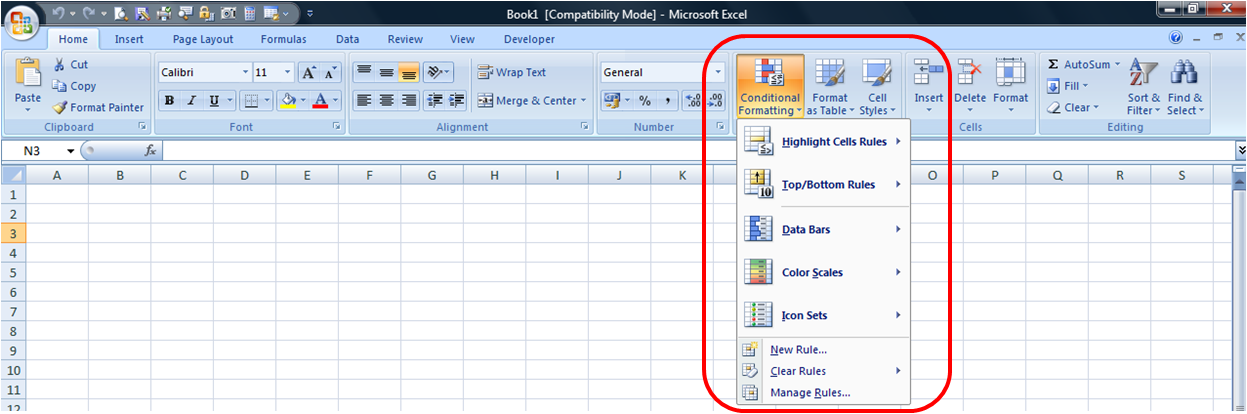
We are not going to detail all of its function and we will demostrate a basic example on this article.

Set Conditional Format To A Cell Based On Cell Content

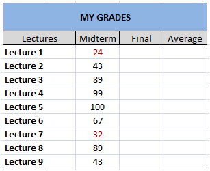
Say that you are planning to make a table for your university grades and we have midtrem grades on this table.

excel

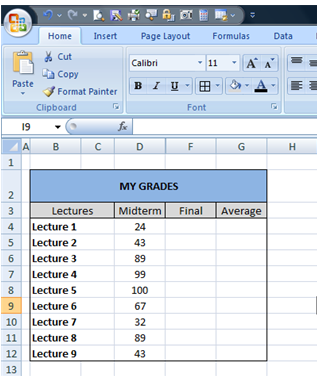
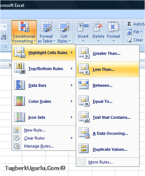
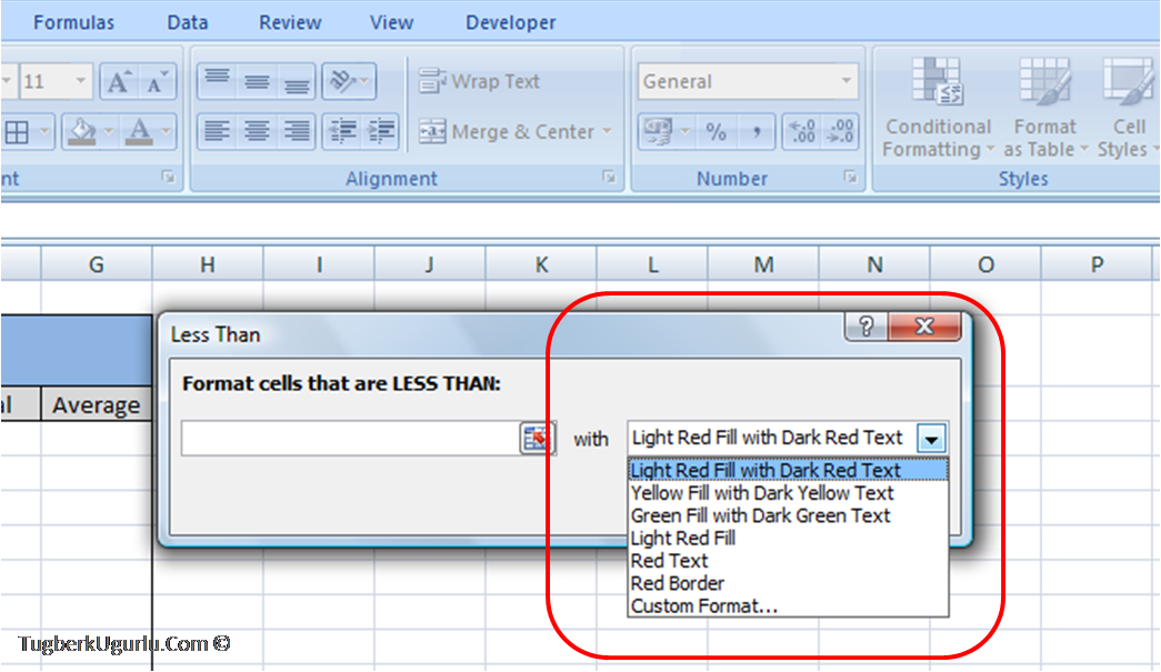
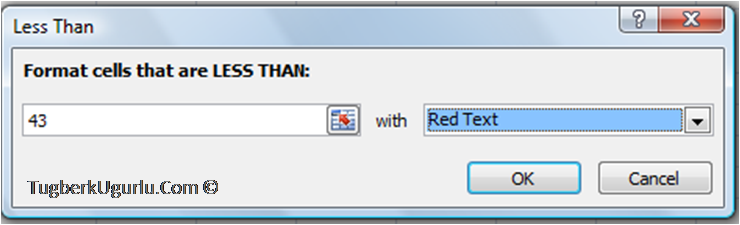
And you want that grades cells under 43 will be shown as red. Before we start, select the cells you wanna set the rules on and follow these steps;

Go to Conditional Formating section on Home part and follow Highlight Cells Rules > Less Than…
And you will see a new window like this:

Let’s dig our this new window. The left box is the place where we will enter our target value which we want it to be our basis value of the rule. On our case, it needs to be 43 because we want the grades being under 43 to be formatted. After we do that, it comes to magic part.
On the right dropdownlist, we will choose or set our rule which we want to set on our target. As soon as you expand it, you will see the values there;

Microsoft Office offers us these values automaticaly. These are most comman used values and we will use Red Text here. After we all do that our window should look like this;

You probably notice Custom Format inside this list. We will not dig out that in this article but that part gives you the ability to be more flexible on your rule.
And then you will see what we have.